import pandas as pd
import numpy as np
import os
import matplotlib.pyplot as plt
from matplotlib.patches import Patch # To manually add legends
import geopandas as gpd
import rioxarray as rioxr
from pystac_client import Client  # To access STAC catalogs
import planetary_computer  # To sign items from the MPC STAC catalog
import contextily as ctx # BasemapsMore content available at the github repository
About
Purpose
Due to a rapid increase in developed land, Phoenix, Arizona has seen changes in biodiversity. In this notebook we investigate the impacts of the increase on biodiversity by analyzing the changes in Biodiversity Intactness Index(BII).
Highlights
- Searching for data using the Microsoft Planetary Computer’s(MPC) STAC API
- Clipping large raster to detailed geometry using
rio.clip() - Map making using
matplotlib
About the data
The first dataset is the Biodiversity Intactness Index(BII) Time Series. This data comes from the Microsoft Planetary Computer STAC catalog. In the analysis we use the 2017 and 2020 rasters.
The second dataset is the Census Bureau County Subdivisions shapefile for Arizona. The Phoenix subdivision was downloaded from this shapefile.
An ESRI National Geographic style world basemap was used to show the Phoenix subdivision in its broader geographic context.
References
Microsoft Planetary Computer. (n.d.). IO biodiversity dataset. Retrieved December 3, 2024, from https://planetarycomputer.microsoft.com/dataset/io-biodiversity
U.S. Census Bureau. (2024). Arizona county subdivisions: tl_2024_04_cousub.shp [Shapefile dataset]. Retrieved from https://www.census.gov/cgi-bin/geo/shapefiles/index.php?year=2024&layergroup=County+Subdivisions
Esri. (n.d.). National Geographic Style [Basemap]. ArcGIS. Retrieved December 6, 2024, from https://hub.arcgis.com/maps/3d1a30626bbc46c582f148b9252676ce/explore【6】.
Import necessary packages
Read in data
# Access MPC catalog
catalog = Client.open(
    "https://planetarycomputer.microsoft.com/api/stac/v1",
    modifier=planetary_computer.sign_inplace,
)
# Import arizona data
fp = os.path.join('data','tl_2024_04_cousub','tl_2024_04_cousub.shp')
az = gpd.read_file(fp)Data exploration
Here we are going to explore the two datasets to familiarize ourselves.
# View the io-biodiversity collection
catalog.get_child('io-biodiversity')- type "Collection"
- id "io-biodiversity"
- stac_version "1.0.0"
- description "Generated by [Impact Observatory](https://www.impactobservatory.com/), in collaboration with [Vizzuality](https://www.vizzuality.com/), these datasets estimate terrestrial Biodiversity Intactness as 100-meter gridded maps for the years 2017-2020. Maps depicting the intactness of global biodiversity have become a critical tool for spatial planning and management, monitoring the extent of biodiversity across Earth, and identifying critical remaining intact habitat. Yet, these maps are often years out of date by the time they are available to scientists and policy-makers. The datasets in this STAC Collection build on past studies that map Biodiversity Intactness using the [PREDICTS database](https://onlinelibrary.wiley.com/doi/full/10.1002/ece3.2579) of spatially referenced observations of biodiversity across 32,000 sites from over 750 studies. The approach differs from previous work by modeling the relationship between observed biodiversity metrics and contemporary, global, geospatial layers of human pressures, with the intention of providing a high resolution monitoring product into the future. Biodiversity intactness is estimated as a combination of two metrics: Abundance, the quantity of individuals, and Compositional Similarity, how similar the composition of species is to an intact baseline. Linear mixed effects models are fit to estimate the predictive capacity of spatial datasets of human pressures on each of these metrics and project results spatially across the globe. These methods, as well as comparisons to other leading datasets and guidance on interpreting results, are further explained in a methods [white paper](https://ai4edatasetspublicassets.blob.core.windows.net/assets/pdfs/io-biodiversity/Biodiversity_Intactness_whitepaper.pdf) entitled “Global 100m Projections of Biodiversity Intactness for the years 2017-2020.” All years are available under a Creative Commons BY-4.0 license. "
links[] 7 items
0
- rel "items"
- href "https://planetarycomputer.microsoft.com/api/stac/v1/collections/io-biodiversity/items"
- type "application/geo+json"
1
- rel "root"
- href "https://planetarycomputer.microsoft.com/api/stac/v1/"
- type "application/json"
- title "Microsoft Planetary Computer STAC API"
2
- rel "license"
- href "https://creativecommons.org/licenses/by/4.0/"
- type "text/html"
- title "CC BY 4.0"
3
- rel "about"
- href "https://ai4edatasetspublicassets.blob.core.windows.net/assets/pdfs/io-biodiversity/Biodiversity_Intactness_whitepaper.pdf"
- type "application/pdf"
- title "Technical White Paper"
4
- rel "describedby"
- href "https://planetarycomputer.microsoft.com/dataset/io-biodiversity"
- type "text/html"
- title "Human readable dataset overview and reference"
5
- rel "self"
- href "https://planetarycomputer.microsoft.com/api/stac/v1/collections/io-biodiversity"
- type "application/json"
6
- rel "parent"
- href "https://planetarycomputer.microsoft.com/api/stac/v1"
- type "application/json"
- title "Microsoft Planetary Computer STAC API"
stac_extensions[] 3 items
- 0 "https://stac-extensions.github.io/item-assets/v1.0.0/schema.json"
- 1 "https://stac-extensions.github.io/raster/v1.1.0/schema.json"
- 2 "https://stac-extensions.github.io/table/v1.2.0/schema.json"
item_assets
data
- type "image/tiff; application=geotiff; profile=cloud-optimized"
roles[] 1 items
- 0 "data"
- title "Biodiversity Intactness"
- description "Terrestrial biodiversity intactness at 100m resolution"
raster:bands[] 1 items
0
- sampling "area"
- data_type "float32"
- spatial_resolution 100
- msft:region "westeurope"
- msft:container "impact"
- msft:storage_account "pcdata01euw"
- msft:short_description "Global terrestrial biodiversity intactness at 100m resolution for years 2017-2020"
- title "Biodiversity Intactness"
extent
spatial
bbox[] 1 items
0[] 4 items
- 0 -180
- 1 -90
- 2 180
- 3 90
temporal
interval[] 1 items
0[] 2 items
- 0 "2017-01-01T00:00:00Z"
- 1 "2020-12-31T23:59:59Z"
- license "CC-BY-4.0"
keywords[] 2 items
- 0 "Global"
- 1 "Biodiversity"
providers[] 3 items
0
- name "Impact Observatory"
roles[] 3 items
- 0 "processor"
- 1 "producer"
- 2 "licensor"
- url "https://www.impactobservatory.com/"
1
- name "Vizzuality"
roles[] 1 items
- 0 "processor"
- url "https://www.vizzuality.com/"
2
- name "Microsoft"
roles[] 1 items
- 0 "host"
- url "https://planetarycomputer.microsoft.com"
summaries
version[] 1 items
- 0 "v1"
assets
thumbnail
- href "https://ai4edatasetspublicassets.blob.core.windows.net/assets/pc_thumbnails/io-biodiversity-thumb.png"
- title "Biodiversity Intactness"
- media_type "image/png"
geoparquet-items
- href "abfs://items/io-biodiversity.parquet"
- type "application/x-parquet"
- title "GeoParquet STAC items"
- description "Snapshot of the collection's STAC items exported to GeoParquet format."
msft:partition_info
- is_partitioned False
table:storage_options
- account_name "pcstacitems"
roles[] 1 items
- 0 "stac-items"
# Create bounding box for search
bbox_of_interest = [-112.826843, 32.974108, -111.184387, 33.863574]
# Create time range for search
time_range = "2017-01-01/2020-01-01"
# Search MPC catalog
search = catalog.search(collections=["io-biodiversity"], bbox=bbox_of_interest, datetime = time_range)
# Retrieve search items
items = search.item_collection()
len(items)4# Look at properties of each items to view the date ranges
items- type "FeatureCollection"
features[] 4 items
0
- type "Feature"
- stac_version "1.0.0"
stac_extensions[] 3 items
- 0 "https://stac-extensions.github.io/projection/v1.0.0/schema.json"
- 1 "https://stac-extensions.github.io/raster/v1.1.0/schema.json"
- 2 "https://stac-extensions.github.io/version/v1.1.0/schema.json"
- id "bii_2020_34.74464974521749_-115.38597824385106_cog"
geometry
- type "Polygon"
coordinates[] 1 items
0[] 9 items
0[] 2 items
- 0 -114.7625474
- 1 27.565314
1[] 2 items
- 0 -108.2066425
- 1 27.565314
2[] 2 items
- 0 -108.2066425
- 1 34.7446497
3[] 2 items
- 0 -115.3859782
- 1 34.7446497
4[] 2 items
- 0 -115.3859782
- 1 29.5649638
5[] 2 items
- 0 -115.3581305
- 1 28.0791503
6[] 2 items
- 0 -115.2036202
- 1 27.8662496
7[] 2 items
- 0 -114.9988044
- 1 27.7099428
8[] 2 items
- 0 -114.7625474
- 1 27.565314
bbox[] 4 items
- 0 -115.3859782
- 1 27.565314
- 2 -108.2066425
- 3 34.7446497
properties
- datetime None
- proj:epsg 4326
proj:shape[] 2 items
- 0 7992
- 1 7992
- end_datetime "2020-12-31T23:59:59Z"
proj:transform[] 9 items
- 0 0.0008983152841195215
- 1 0.0
- 2 -115.38597824385106
- 3 0.0
- 4 -0.0008983152841195215
- 5 34.74464974521749
- 6 0.0
- 7 0.0
- 8 1.0
- start_datetime "2020-01-01T00:00:00Z"
links[] 5 items
0
- rel "collection"
- href "https://planetarycomputer.microsoft.com/api/stac/v1/collections/io-biodiversity"
- type "application/json"
1
- rel "parent"
- href "https://planetarycomputer.microsoft.com/api/stac/v1/collections/io-biodiversity"
- type "application/json"
2
- rel "root"
- href "https://planetarycomputer.microsoft.com/api/stac/v1"
- type "application/json"
- title "Microsoft Planetary Computer STAC API"
3
- rel "self"
- href "https://planetarycomputer.microsoft.com/api/stac/v1/collections/io-biodiversity/items/bii_2020_34.74464974521749_-115.38597824385106_cog"
- type "application/geo+json"
4
- rel "preview"
- href "https://planetarycomputer.microsoft.com/api/data/v1/item/map?collection=io-biodiversity&item=bii_2020_34.74464974521749_-115.38597824385106_cog"
- type "text/html"
- title "Map of item"
assets
data
- href "https://pcdata01euw.blob.core.windows.net/impact/bii-v1/bii_2020/bii_2020_34.74464974521749_-115.38597824385106_cog.tif?st=2024-12-05T18%3A59%3A04Z&se=2024-12-06T19%3A44%3A04Z&sp=rl&sv=2024-05-04&sr=c&skoid=9c8ff44a-6a2c-4dfb-b298-1c9212f64d9a&sktid=72f988bf-86f1-41af-91ab-2d7cd011db47&skt=2024-12-06T14%3A30%3A01Z&ske=2024-12-13T14%3A30%3A01Z&sks=b&skv=2024-05-04&sig=B5lhKIHtISXzYwusPjA3ITMKGC76PEs2osWN295mCzw%3D"
- type "image/tiff; application=geotiff; profile=cloud-optimized"
- title "Biodiversity Intactness"
- description "Terrestrial biodiversity intactness at 100m resolution"
- version "v1"
raster:bands[] 1 items
0
- sampling "area"
- data_type "float32"
- spatial_resolution 100
roles[] 1 items
- 0 "data"
tilejson
- href "https://planetarycomputer.microsoft.com/api/data/v1/item/tilejson.json?collection=io-biodiversity&item=bii_2020_34.74464974521749_-115.38597824385106_cog&assets=data&tile_format=png&colormap_name=io-bii&rescale=0%2C1&expression=0.97%2A%28data_b1%2A%2A3.84%29&format=png"
- type "application/json"
- title "TileJSON with default rendering"
roles[] 1 items
- 0 "tiles"
rendered_preview
- href "https://planetarycomputer.microsoft.com/api/data/v1/item/preview.png?collection=io-biodiversity&item=bii_2020_34.74464974521749_-115.38597824385106_cog&assets=data&tile_format=png&colormap_name=io-bii&rescale=0%2C1&expression=0.97%2A%28data_b1%2A%2A3.84%29&format=png"
- type "image/png"
- title "Rendered preview"
- rel "preview"
roles[] 1 items
- 0 "overview"
- collection "io-biodiversity"
1
- type "Feature"
- stac_version "1.0.0"
stac_extensions[] 3 items
- 0 "https://stac-extensions.github.io/projection/v1.0.0/schema.json"
- 1 "https://stac-extensions.github.io/raster/v1.1.0/schema.json"
- 2 "https://stac-extensions.github.io/version/v1.1.0/schema.json"
- id "bii_2019_34.74464974521749_-115.38597824385106_cog"
geometry
- type "Polygon"
coordinates[] 1 items
0[] 10 items
0[] 2 items
- 0 -114.7625474
- 1 27.565314
1[] 2 items
- 0 -108.2066425
- 1 27.565314
2[] 2 items
- 0 -108.2066425
- 1 34.7446497
3[] 2 items
- 0 -115.3859782
- 1 34.7446497
4[] 2 items
- 0 -115.3859782
- 1 29.5649638
5[] 2 items
- 0 -115.3581305
- 1 28.0791503
6[] 2 items
- 0 -115.2161967
- 1 27.8761311
7[] 2 items
- 0 -115.0068892
- 1 27.7180276
8[] 2 items
- 0 -114.8469891
- 1 27.6174163
9[] 2 items
- 0 -114.7625474
- 1 27.565314
bbox[] 4 items
- 0 -115.3859782
- 1 27.565314
- 2 -108.2066425
- 3 34.7446497
properties
- datetime None
- proj:epsg 4326
proj:shape[] 2 items
- 0 7992
- 1 7992
- end_datetime "2019-12-31T23:59:59Z"
proj:transform[] 9 items
- 0 0.0008983152841195215
- 1 0.0
- 2 -115.38597824385106
- 3 0.0
- 4 -0.0008983152841195215
- 5 34.74464974521749
- 6 0.0
- 7 0.0
- 8 1.0
- start_datetime "2019-01-01T00:00:00Z"
links[] 5 items
0
- rel "collection"
- href "https://planetarycomputer.microsoft.com/api/stac/v1/collections/io-biodiversity"
- type "application/json"
1
- rel "parent"
- href "https://planetarycomputer.microsoft.com/api/stac/v1/collections/io-biodiversity"
- type "application/json"
2
- rel "root"
- href "https://planetarycomputer.microsoft.com/api/stac/v1"
- type "application/json"
- title "Microsoft Planetary Computer STAC API"
3
- rel "self"
- href "https://planetarycomputer.microsoft.com/api/stac/v1/collections/io-biodiversity/items/bii_2019_34.74464974521749_-115.38597824385106_cog"
- type "application/geo+json"
4
- rel "preview"
- href "https://planetarycomputer.microsoft.com/api/data/v1/item/map?collection=io-biodiversity&item=bii_2019_34.74464974521749_-115.38597824385106_cog"
- type "text/html"
- title "Map of item"
assets
data
- href "https://pcdata01euw.blob.core.windows.net/impact/bii-v1/bii_2019/bii_2019_34.74464974521749_-115.38597824385106_cog.tif?st=2024-12-05T18%3A59%3A04Z&se=2024-12-06T19%3A44%3A04Z&sp=rl&sv=2024-05-04&sr=c&skoid=9c8ff44a-6a2c-4dfb-b298-1c9212f64d9a&sktid=72f988bf-86f1-41af-91ab-2d7cd011db47&skt=2024-12-06T14%3A30%3A01Z&ske=2024-12-13T14%3A30%3A01Z&sks=b&skv=2024-05-04&sig=B5lhKIHtISXzYwusPjA3ITMKGC76PEs2osWN295mCzw%3D"
- type "image/tiff; application=geotiff; profile=cloud-optimized"
- title "Biodiversity Intactness"
- description "Terrestrial biodiversity intactness at 100m resolution"
- version "v1"
raster:bands[] 1 items
0
- sampling "area"
- data_type "float32"
- spatial_resolution 100
roles[] 1 items
- 0 "data"
tilejson
- href "https://planetarycomputer.microsoft.com/api/data/v1/item/tilejson.json?collection=io-biodiversity&item=bii_2019_34.74464974521749_-115.38597824385106_cog&assets=data&tile_format=png&colormap_name=io-bii&rescale=0%2C1&expression=0.97%2A%28data_b1%2A%2A3.84%29&format=png"
- type "application/json"
- title "TileJSON with default rendering"
roles[] 1 items
- 0 "tiles"
rendered_preview
- href "https://planetarycomputer.microsoft.com/api/data/v1/item/preview.png?collection=io-biodiversity&item=bii_2019_34.74464974521749_-115.38597824385106_cog&assets=data&tile_format=png&colormap_name=io-bii&rescale=0%2C1&expression=0.97%2A%28data_b1%2A%2A3.84%29&format=png"
- type "image/png"
- title "Rendered preview"
- rel "preview"
roles[] 1 items
- 0 "overview"
- collection "io-biodiversity"
2
- type "Feature"
- stac_version "1.0.0"
stac_extensions[] 3 items
- 0 "https://stac-extensions.github.io/projection/v1.0.0/schema.json"
- 1 "https://stac-extensions.github.io/raster/v1.1.0/schema.json"
- 2 "https://stac-extensions.github.io/version/v1.1.0/schema.json"
- id "bii_2018_34.74464974521749_-115.38597824385106_cog"
geometry
- type "Polygon"
coordinates[] 1 items
0[] 10 items
0[] 2 items
- 0 -114.7625474
- 1 27.565314
1[] 2 items
- 0 -108.2066425
- 1 27.565314
2[] 2 items
- 0 -108.2066425
- 1 34.7446497
3[] 2 items
- 0 -115.3859782
- 1 34.7446497
4[] 2 items
- 0 -115.3859782
- 1 29.5649638
5[] 2 items
- 0 -115.3581305
- 1 28.0791503
6[] 2 items
- 0 -115.2179933
- 1 27.8869109
7[] 2 items
- 0 -115.1775691
- 1 27.8491816
8[] 2 items
- 0 -115.0014993
- 1 27.7117394
9[] 2 items
- 0 -114.7625474
- 1 27.565314
bbox[] 4 items
- 0 -115.3859782
- 1 27.565314
- 2 -108.2066425
- 3 34.7446497
properties
- datetime None
- proj:epsg 4326
proj:shape[] 2 items
- 0 7992
- 1 7992
- end_datetime "2018-12-31T23:59:59Z"
proj:transform[] 9 items
- 0 0.0008983152841195215
- 1 0.0
- 2 -115.38597824385106
- 3 0.0
- 4 -0.0008983152841195215
- 5 34.74464974521749
- 6 0.0
- 7 0.0
- 8 1.0
- start_datetime "2018-01-01T00:00:00Z"
links[] 5 items
0
- rel "collection"
- href "https://planetarycomputer.microsoft.com/api/stac/v1/collections/io-biodiversity"
- type "application/json"
1
- rel "parent"
- href "https://planetarycomputer.microsoft.com/api/stac/v1/collections/io-biodiversity"
- type "application/json"
2
- rel "root"
- href "https://planetarycomputer.microsoft.com/api/stac/v1"
- type "application/json"
- title "Microsoft Planetary Computer STAC API"
3
- rel "self"
- href "https://planetarycomputer.microsoft.com/api/stac/v1/collections/io-biodiversity/items/bii_2018_34.74464974521749_-115.38597824385106_cog"
- type "application/geo+json"
4
- rel "preview"
- href "https://planetarycomputer.microsoft.com/api/data/v1/item/map?collection=io-biodiversity&item=bii_2018_34.74464974521749_-115.38597824385106_cog"
- type "text/html"
- title "Map of item"
assets
data
- href "https://pcdata01euw.blob.core.windows.net/impact/bii-v1/bii_2018/bii_2018_34.74464974521749_-115.38597824385106_cog.tif?st=2024-12-05T18%3A59%3A04Z&se=2024-12-06T19%3A44%3A04Z&sp=rl&sv=2024-05-04&sr=c&skoid=9c8ff44a-6a2c-4dfb-b298-1c9212f64d9a&sktid=72f988bf-86f1-41af-91ab-2d7cd011db47&skt=2024-12-06T14%3A30%3A01Z&ske=2024-12-13T14%3A30%3A01Z&sks=b&skv=2024-05-04&sig=B5lhKIHtISXzYwusPjA3ITMKGC76PEs2osWN295mCzw%3D"
- type "image/tiff; application=geotiff; profile=cloud-optimized"
- title "Biodiversity Intactness"
- description "Terrestrial biodiversity intactness at 100m resolution"
- version "v1"
raster:bands[] 1 items
0
- sampling "area"
- data_type "float32"
- spatial_resolution 100
roles[] 1 items
- 0 "data"
tilejson
- href "https://planetarycomputer.microsoft.com/api/data/v1/item/tilejson.json?collection=io-biodiversity&item=bii_2018_34.74464974521749_-115.38597824385106_cog&assets=data&tile_format=png&colormap_name=io-bii&rescale=0%2C1&expression=0.97%2A%28data_b1%2A%2A3.84%29&format=png"
- type "application/json"
- title "TileJSON with default rendering"
roles[] 1 items
- 0 "tiles"
rendered_preview
- href "https://planetarycomputer.microsoft.com/api/data/v1/item/preview.png?collection=io-biodiversity&item=bii_2018_34.74464974521749_-115.38597824385106_cog&assets=data&tile_format=png&colormap_name=io-bii&rescale=0%2C1&expression=0.97%2A%28data_b1%2A%2A3.84%29&format=png"
- type "image/png"
- title "Rendered preview"
- rel "preview"
roles[] 1 items
- 0 "overview"
- collection "io-biodiversity"
3
- type "Feature"
- stac_version "1.0.0"
stac_extensions[] 3 items
- 0 "https://stac-extensions.github.io/projection/v1.0.0/schema.json"
- 1 "https://stac-extensions.github.io/raster/v1.1.0/schema.json"
- 2 "https://stac-extensions.github.io/version/v1.1.0/schema.json"
- id "bii_2017_34.74464974521749_-115.38597824385106_cog"
geometry
- type "Polygon"
coordinates[] 1 items
0[] 10 items
0[] 2 items
- 0 -114.7616491
- 1 27.565314
1[] 2 items
- 0 -108.2066425
- 1 27.565314
2[] 2 items
- 0 -108.2066425
- 1 34.7446497
3[] 2 items
- 0 -115.3859782
- 1 34.7446497
4[] 2 items
- 0 -115.3859782
- 1 29.5649638
5[] 2 items
- 0 -115.3581305
- 1 28.0791503
6[] 2 items
- 0 -115.2036202
- 1 27.8662496
7[] 2 items
- 0 -115.0068892
- 1 27.7180276
8[] 2 items
- 0 -114.8469891
- 1 27.6174163
9[] 2 items
- 0 -114.7616491
- 1 27.565314
bbox[] 4 items
- 0 -115.3859782
- 1 27.565314
- 2 -108.2066425
- 3 34.7446497
properties
- datetime None
- proj:epsg 4326
proj:shape[] 2 items
- 0 7992
- 1 7992
- end_datetime "2017-12-31T23:59:59Z"
proj:transform[] 9 items
- 0 0.0008983152841195215
- 1 0.0
- 2 -115.38597824385106
- 3 0.0
- 4 -0.0008983152841195215
- 5 34.74464974521749
- 6 0.0
- 7 0.0
- 8 1.0
- start_datetime "2017-01-01T00:00:00Z"
links[] 5 items
0
- rel "collection"
- href "https://planetarycomputer.microsoft.com/api/stac/v1/collections/io-biodiversity"
- type "application/json"
1
- rel "parent"
- href "https://planetarycomputer.microsoft.com/api/stac/v1/collections/io-biodiversity"
- type "application/json"
2
- rel "root"
- href "https://planetarycomputer.microsoft.com/api/stac/v1"
- type "application/json"
- title "Microsoft Planetary Computer STAC API"
3
- rel "self"
- href "https://planetarycomputer.microsoft.com/api/stac/v1/collections/io-biodiversity/items/bii_2017_34.74464974521749_-115.38597824385106_cog"
- type "application/geo+json"
4
- rel "preview"
- href "https://planetarycomputer.microsoft.com/api/data/v1/item/map?collection=io-biodiversity&item=bii_2017_34.74464974521749_-115.38597824385106_cog"
- type "text/html"
- title "Map of item"
assets
data
- href "https://pcdata01euw.blob.core.windows.net/impact/bii-v1/bii_2017/bii_2017_34.74464974521749_-115.38597824385106_cog.tif?st=2024-12-05T18%3A59%3A04Z&se=2024-12-06T19%3A44%3A04Z&sp=rl&sv=2024-05-04&sr=c&skoid=9c8ff44a-6a2c-4dfb-b298-1c9212f64d9a&sktid=72f988bf-86f1-41af-91ab-2d7cd011db47&skt=2024-12-06T14%3A30%3A01Z&ske=2024-12-13T14%3A30%3A01Z&sks=b&skv=2024-05-04&sig=B5lhKIHtISXzYwusPjA3ITMKGC76PEs2osWN295mCzw%3D"
- type "image/tiff; application=geotiff; profile=cloud-optimized"
- title "Biodiversity Intactness"
- description "Terrestrial biodiversity intactness at 100m resolution"
- version "v1"
raster:bands[] 1 items
0
- sampling "area"
- data_type "float32"
- spatial_resolution 100
roles[] 1 items
- 0 "data"
tilejson
- href "https://planetarycomputer.microsoft.com/api/data/v1/item/tilejson.json?collection=io-biodiversity&item=bii_2017_34.74464974521749_-115.38597824385106_cog&assets=data&tile_format=png&colormap_name=io-bii&rescale=0%2C1&expression=0.97%2A%28data_b1%2A%2A3.84%29&format=png"
- type "application/json"
- title "TileJSON with default rendering"
roles[] 1 items
- 0 "tiles"
rendered_preview
- href "https://planetarycomputer.microsoft.com/api/data/v1/item/preview.png?collection=io-biodiversity&item=bii_2017_34.74464974521749_-115.38597824385106_cog&assets=data&tile_format=png&colormap_name=io-bii&rescale=0%2C1&expression=0.97%2A%28data_b1%2A%2A3.84%29&format=png"
- type "image/png"
- title "Rendered preview"
- rel "preview"
roles[] 1 items
- 0 "overview"
- collection "io-biodiversity"
# Select unique search item
item_20 = items[0]
item_17 = items[3]
# View the properties of the item to view the projection
print('id:' , item_17.id)
item_17.propertiesid: bii_2017_34.74464974521749_-115.38597824385106_cog{'datetime': None,
'proj:epsg': 4326,
'proj:shape': [7992, 7992],
'end_datetime': '2017-12-31T23:59:59Z',
'proj:transform': [0.0008983152841195215,
0.0,
-115.38597824385106,
0.0,
-0.0008983152841195215,
34.74464974521749,
0.0,
0.0,
1.0],
'start_datetime': '2017-01-01T00:00:00Z'}# View the properties of the item to view the projection
print('id:' , item_20.id)
item_20.propertiesid: bii_2020_34.74464974521749_-115.38597824385106_cog{'datetime': None,
'proj:epsg': 4326,
'proj:shape': [7992, 7992],
'end_datetime': '2020-12-31T23:59:59Z',
'proj:transform': [0.0008983152841195215,
0.0,
-115.38597824385106,
0.0,
-0.0008983152841195215,
34.74464974521749,
0.0,
0.0,
1.0],
'start_datetime': '2020-01-01T00:00:00Z'}# Check assets in each item
for key in item_17.assets.keys():
print(key, '--', item_17.assets[key].title)
for key in item_20.assets.keys():
print(key, '--', item_20.assets[key].title)data -- Biodiversity Intactness
tilejson -- TileJSON with default rendering
rendered_preview -- Rendered preview
data -- Biodiversity Intactness
tilejson -- TileJSON with default rendering
rendered_preview -- Rendered previewThe exploration of the MPC STAC catalog gave lots of information. First, we viewed the io-biodiversity collection and were able to obtain its description, temporal extent, spatial extent and more. The temporal extent was 2017-01-01T00:00:00Z - 2020-12-31T23:59:59Z and the spatial extent was [-180, -90, 180, 90]. We then searched the catalog for the collection, date range, and area of interest and found there were 4 items that matched the search. After viewing the 4 items we chose the two of interest, for years 2017 and 2020. We then used .properties to find the projection of each item which was EPSG 4326, and utilizes .assets.keys() to check the assets in each item.
# View the size of the arizona df
az.shape
(80, 17)# View the columns of the arizona df
az.head(3)| STATEFP | COUNTYFP | COUSUBFP | COUSUBNS | GEOID | GEOIDFQ | NAME | NAMELSAD | LSAD | CLASSFP | MTFCC | FUNCSTAT | ALAND | AWATER | INTPTLAT | INTPTLON | geometry | |
|---|---|---|---|---|---|---|---|---|---|---|---|---|---|---|---|---|---|
| 0 | 04 | 005 | 91198 | 01934931 | 0400591198 | 0600000US0400591198 | Flagstaff | Flagstaff CCD | 22 | Z5 | G4040 | S | 12231962349 | 44576380 | +35.1066122 | -111.3662507 | POLYGON ((-112.13370 35.85596, -112.13368 35.8... |
| 1 | 04 | 005 | 91838 | 01934953 | 0400591838 | 0600000US0400591838 | Kaibab Plateau | Kaibab Plateau CCD | 22 | Z5 | G4040 | S | 7228864156 | 29327221 | +36.5991097 | -112.1368033 | POLYGON ((-112.66039 36.53941, -112.66033 36.5... |
| 2 | 04 | 005 | 91683 | 01934950 | 0400591683 | 0600000US0400591683 | Hualapai | Hualapai CCD | 22 | Z5 | G4040 | S | 2342313339 | 3772690 | +35.9271665 | -113.1170408 | POLYGON ((-113.35416 36.04097, -113.35416 36.0... |
# Filter arizona df to Phoenix subdivision
phx = az[az['NAME'] == "Phoenix"]
phx.head()| STATEFP | COUNTYFP | COUSUBFP | COUSUBNS | GEOID | GEOIDFQ | NAME | NAMELSAD | LSAD | CLASSFP | MTFCC | FUNCSTAT | ALAND | AWATER | INTPTLAT | INTPTLON | geometry | |
|---|---|---|---|---|---|---|---|---|---|---|---|---|---|---|---|---|---|
| 10 | 04 | 013 | 92601 | 01934968 | 0401392601 | 0600000US0401392601 | Phoenix | Phoenix CCD | 22 | Z5 | G4040 | S | 2806483087 | 9458600 | +33.5211331 | -112.0284405 | POLYGON ((-112.47014 33.55996, -112.47011 33.5... |
By exploring the shape of the Arizona df we found there were 80 rows and 17 columns. We then viewed the first three rows of the df. After this we were able to use the column names to filter the df to just the Phoenix subdivision. We viewed the new Phoenix df to ensure only Phoenix was present, and one row matched the filter.
Phoenix, AZ Map
Create a map showing where Phoenix is located in Arizona.
fig, ax = plt.subplots(figsize = (10, 10))
ax.axis('off')

phx.plot(ax=ax, alpha = 0.4, facecolor = "#b2182b",  edgecolor = "black") # Add transparent phoenix polygon

ctx.add_basemap(ax=ax, source=ctx.providers.Esri.NatGeoWorldMap, crs=phx.crs) # Add basemap with contextily

plt.title('Phoenix Subdivision in Arizona', fontsize = 16)

legend = [Patch(facecolor = '#b2182b', alpha = 0.4, edgecolor = 'black', label = 'Phoenix subdivision')] # Manually add legend
ax.legend(handles=legend)

plt.savefig('images/phoenix_arizona_map.png') # Save map in images folder
plt.show()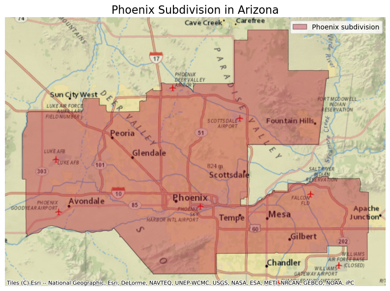
Visualizing BII loss in Phoenix
We want to find the percent area in Phoenix with a BII greater than or equal to 0.75 in the years 2017 and 2020.
# Open the raster data
bii17 = rioxr.open_rasterio(item_17.assets['data'].href)
bii20 = rioxr.open_rasterio(item_20.assets['data'].href)
# Clip the bii rasters to phoenix
bii17_phx = bii17.rio.clip(phx['geometry'])
bii20_phx = bii20.rio.clip(phx['geometry'])# Find areas where bii >= 0.75 and assign 1 to true and 0 to false
bii17_high = (bii17_phx >= 0.75).astype('int')
bii20_high = (bii20_phx >= 0.75).astype('int')# Find total number of pixels for each year
total_pix_17 = bii17_phx.count().item()
total_pix_20 = bii20_phx.count().item()# Find count of pixels above 0.75 bii for each year
bii_pix_17 = bii17_high.values.sum()
bii_pix_20 = bii20_high.values.sum()# Calculate percentages
bii_pct17 = (bii_pix_17 / total_pix_17) * 100
bii_pct20 = (bii_pix_20 / total_pix_20) * 100
print(f"In 2017, {round(bii_pct17, 2)}% of the Phoenix subdivision had a BII of at least 0.75" )
print(f"In 2020, {round(bii_pct20, 2)}% of the Phoenix subdivision had a BII of at least 0.75" )In 2017, 7.13% of the Phoenix subdivision had a BII of at least 0.75
In 2020, 6.49% of the Phoenix subdivision had a BII of at least 0.75BII lost from 2017 to 2020
There was a higher percent of area in Phoenix with a BII of at least 0.75 in 2017 than in 2020. We want to create a visualization showing the areas that fell below this threshold between the two years. We can do this by subtracting the 2020 pixels from the 2017 pixels where BII ≥ 0.75.
# Calculate difference in pixels above 0.75 from 2017 to 2020
diff_17_20 = bii17_high - bii20_high

# Set all that are not 1 to na
loss_17_20 = diff_17_20.where(diff_17_20 == 1)
# Create map
fig, ax = plt.subplots(figsize = (10, 10)) # Set figure size
ax.axis('off')
bii20_phx.plot(ax=ax, cmap = 'Greens', cbar_kwargs={'orientation':'horizontal', 'label':'BII for 2020'}) # Plot BII for 2020
loss_17_20.plot(ax=ax, cmap = 'brg', add_colorbar = False) # Plot BII that fell below threshold
phx.plot(ax = ax, color = "none", edgecolor = "black", linewidth = 0.75) # Add outline to phx polygon
legend = [Patch(facecolor = 'red', label = 'Area with BII ≥ 0.75 lost from 2017 to 2020')] # Manually add legend
ax.legend(handles=legend, loc=(0.25, -0.2)) # Legend
ax.set_title("Biodiversity Intactness Index (BII)\nPhoenix Subdivision")
plt.savefig('images/bii_phoenix.png') # Save map in images folder
plt.show()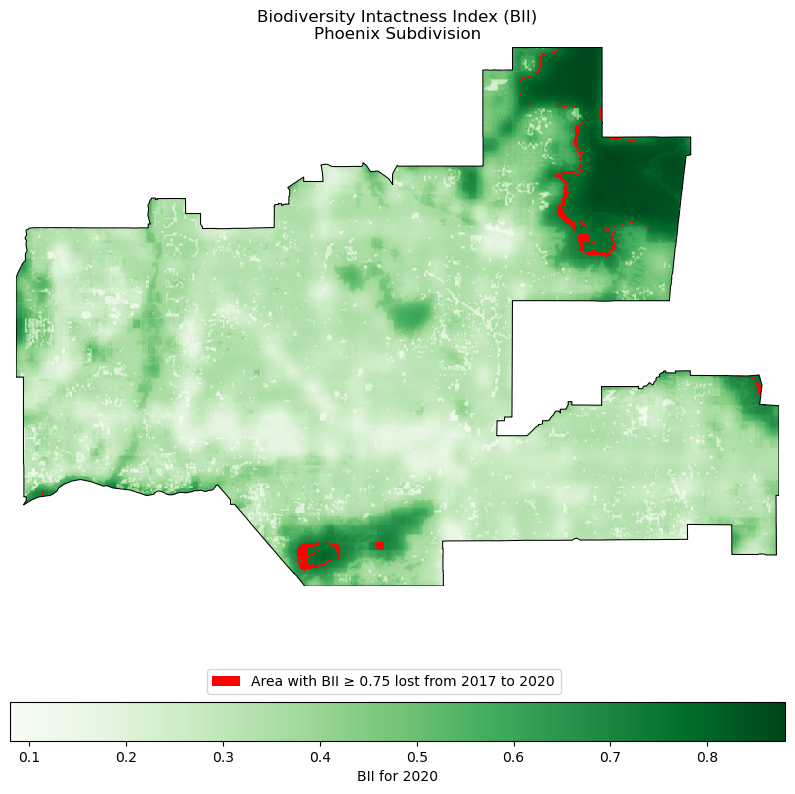
Our calculations above told us that almost 1% of the Phoenix area previously had a BII of above 0.75 in 2017, and by 2020 fell below that threshold. From the map, we can visualize where that 1% is located, highlighted in red. The map also shows us that a high area of the phoenix subdivision falls below a BII of 0.3. A very small portion of Phoenix has a BII of 0.6 or higher, helping us visualize the negative effects of rapid urban sprawl on biodiversity.